
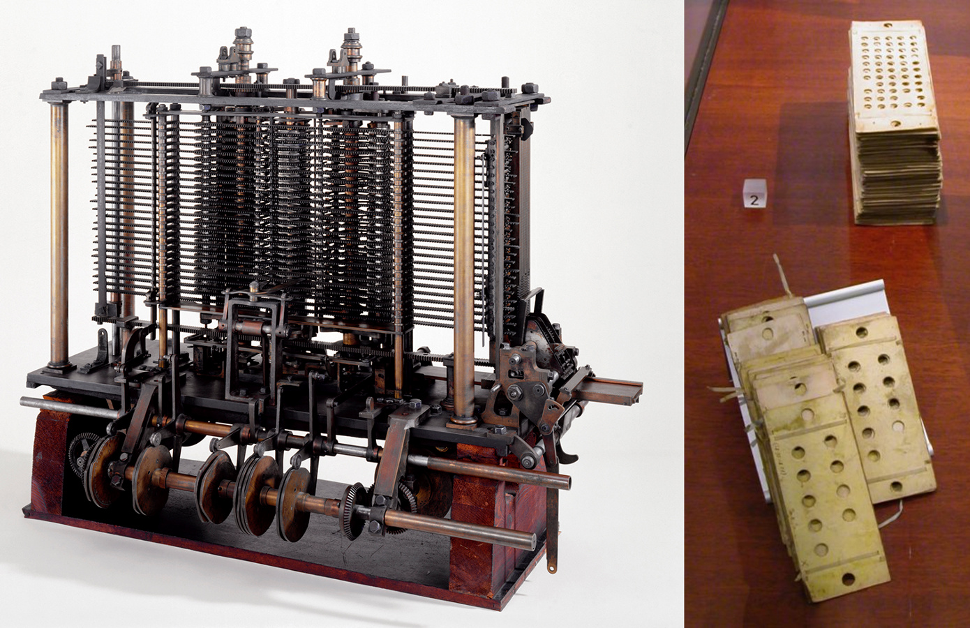
Fragment of the Analytical Engine’s arithmetic/logic unit built by Babbage (photo: Science Museum London) and punched cards for operating it (photo: Karoly Lorentey)
Following on from my post about his Difference Engine, Charles Babbage’s Analytical Engine deserves some discussion. Only small pieces of the Analytical Engine were built. Indeed, Babbage’s ideas were so far ahead of his time that it could not be built with the technology available to him. Babbage was clearly either a true genius – or else he was a time-traveller from the future trying to recreate a modern computer.
It is not quite clear whether Babbage’s Analytical Engine was Turing complete. The kind of abstract computer developed independently by Alan Turing and Emil Post uses an arbitrarily long tape. Even more abstract models of computation use arbitrarily long integers to achieve the same effect. For example, the list (2, 3, 0, 1) can be encoded as the number 582 (1001000110 in binary). Modern computers use a sequence of numbered memory locations, accessed by indexing. The Analytical Engine could not do this. To quote the excellent analysis by Allan G. Bromley, “With hindsight we may note that in the Analytical Engine (at least until 1840) Babbage did not possess the variable-address concept; that is, there was no mechanism by which the machine could, as a result of a calculation, specify a particular variable in the store to be used as the operand for an instruction.”

Babbage was not terribly good at explaining his ideas in writing, unfortunately. The best description is a 13-page summary of of a lecture by Babbage written in French by Luigi Federico Menabrea (later Prime Minister of Italy). This was translated into English in 1843 by Augusta Ada King-Noel (née Byron), the Countess of Lovelace.
Ada added 36 pages of detailed notes of her own. These include several insightful comments regarding the philosophy of computing, such as: “Again, it might act upon other things besides number, were objects found whose mutual fundamental relations could be expressed by those of the abstract science of operations, and which should be also susceptible of adaptations to the action of the operating notation and mechanism of the engine. Supposing, for instance, that the fundamental relations of pitched sounds in the science of harmony and of musical composition were susceptible of such expression and adaptations, the engine might compose elaborate and scientific pieces of music of any degree of complexity or extent. The Analytical Engine is an embodying of the science of operations, constructed with peculiar reference to abstract number as the subject of those operations.” (from Note A).
Also: “The Analytical Engine has no pretensions whatever to originate anything. It can do whatever we know how to order it to perform.” (from Note G).

Ada is sometimes described as the “first computer programmer,” based on the material in her Note G. This is clearly incorrect, since Charles Babbage had written several dozen programs for the Analytical Engine before 1840. Perhaps “first computer scientist” would be a better title. The program described in Ada’s Note G computes Bernoulli numbers. It does so using the fact that each Bernoulli number can be computed from its predecessors via the relationship:
Here each Ai can be calculated as follows:
a <- function (n, i) {
	if (i == 0) -0.5 * (2*n - 1) / (2*n + 1)
	else if (i == 1) n
	else a(n, i-2) * (2*n + 2 - i) * (2*n + 1 - i) / (i * (i + 1))
}
Bromley notes that “the ‘user instruction set’ of the Analytical Engine seems nowhere to be clearly stated,” which makes it a little difficult to extract an actual program from Ada’s material. After fixing three small bugs, here is something that actually works (in the language R, and all done using numbered registers):
ada <- function (n.max) {
	b <- rep(0, n.max)  # result registers
	v <- c(1, 2, 1, 0, 0, 0, 0, 0, 0, 0, 0, 0, 0)  # other registers

	while (v[3] <= n.max) {  # how is this loop done in the Analytical Engine?
		v[4] <- v[5] <- v[6] <- v[2] * v[3]
		v[4] <- v[4] - v[1]  # v[1] is always 1
		v[5] <- v[5] + v[1]
		v[11] <- v[4] / v[5]  # accidentally reversed in Ada’s diagram
		v[11] <- v[11] / v[2]  # v[2] is always 2
		v[13] <- v[13] - v[11]
		v[10] <- v[3] - v[1]

		if (v[10] > 0) {  # how is this conditional execution done in the Analytical Engine?
			v[7] <- v[2] + v[7]
			v[11] <- v[6] / v[7]
			v[12] <- b[1] * v[11]
			v[13] <- v[12] + v[13]
			v[10] <- v[10] - v[1]
		}

		while(v[10] > 0) {  # how is this loop done in the Analytical Engine?
			v[6] <- v[6] - v[1]
			v[7] <- v[1] + v[7]
			v[8] <- v[6] / v[7]
			v[11] <- v[8] * v[11]
			v[6] <- v[6] - v[1]
			v[7] <- v[1] + v[7]
			v[9] <- v[6] / v[7]
			v[11] <- v[9] * v[11]

			i <- v[3] - v[10]   # how is this indexing done in the Analytical Engine?
			v[12] <- b[i] * v[11]
			v[13] <- v[12] + v[13]
			v[10] <- v[10] - v[1]
		}

		n <- v[3]  # how is this indexing done in the Analytical Engine?
		b[n] <- b[n] - v[13]  # another apparent error in Ada's table at line 14 (negation is needed)

		v[3] <- v[1] + v[3]
		v[7] <- 0   # reset the register with a “variable card”
		v[13] <- 0  # a third apparent error in Ada's table (v[13] needs to be reset, not v[6])
	}
	b
}
There are a number of questions about this. First, I am assuming that all registers are read non-destructively (Ada’s notes indicate that read-and-clear is also possible). Second, the results stored in b require indexing, which the Analytical Engine could not do. Third, Ada writes that “Operation 7 must either bring out a result equal to zero (if n = 1); or a result greater than zero, as in the present case; and the engine follows the one or the other of the two courses just explained, contingently on the one or the other result of Operation 7.” This implies that some kind of conditional branching was possible. But how?
A simple response is simply to “unroll” the loops, breaking the program down into instructions of just three kinds:
Set 1 567: place the number 567 in register #1Do 2 + 3: add the contents of register #2 to the content of register #3 (and similarly for −, ×, and ÷)Store 4: store a previously computed result in register #4
The following, rather lengthy, version of the program correctly computes the first three Bernoulli numbers:
Set 1 1, Set 2 2, Set 3 1

# First Bernoulli number
Do 2 * 3, Store 4, Store 5, Store 6
Do 4 - 1, Store 4
Do 5 + 1, Store 5
Do 4 / 5, Store 11
Do 11 / 2, Store 11
Do 13 - 11, Store 13
Do 3 - 1, Store 10

Do 1 + 3, Store 3
Do 21 - 13, Store 21,  # 21 done
Set 7 0, Set 13 0

# Second Bernoulli number
Do 2 * 3, Store 4, Store 5, Store 6
Do 4 - 1, Store 4
Do 5 + 1, Store 5
Do 4 / 5, Store 11
Do 11 / 2, Store 11
Do 13 - 11, Store 13
Do 3 - 1, Store 10

Do 2 + 7, Store 7
Do 6 / 7, Store 11
Do 21 * 11, Store 12,  # use 21
Do 12 + 13, Store 13
Do 10 - 1, Store 10

Do 1 + 3, Store 3
Do 22 - 13, Store 22,  # 22 done
Set 7 0, Set 13 0

# Third Bernoulli number
Do 2 * 3, Store 4, Store 5, Store 6
Do 4 - 1, Store 4
Do 5 + 1, Store 5
Do 4 / 5, Store 11
Do 11 / 2, Store 11
Do 13 - 11, Store 13
Do 3 - 1, Store 10

Do 2 + 7, Store 7
Do 6 / 7, Store 11
Do 21 * 11, Store 12,  # use 21
Do 12 + 13, Store 13
Do 10 - 1, Store 10

# Inner loop
Do 6 - 1, Store 6
Do 1 + 7, Store 7
Do 6 / 7, Store 8
Do 8 * 11, Store 11
Do 6 - 1, Store 6
Do 1 + 7, Store 7
Do 6 / 7, Store 9
Do 9 * 11, Store 11
Do 22 * 11, Store 12,  # use 22
Do 12 + 13, Store 13
Do 10 - 1, Store 10

Do 1 + 3, Store 3
Do 23 - 13, Store 23,  # 23 done
Set 7 0, Set 13 0
Can we do better than that? Bromley notes that “the mechanism by which the sequencing of operations is obtained is obscure.” Furthermore, driven by what was probably a correct intuition about code/data separation, Babbage separated operation and variable cards, and this would have played havoc with control flow (Bromley again: “I am not convinced that Babbage had clearly resolved even the representational difficulties that his separation of operation and variable cards implies”).
I’m resolving those issues by straying into what Babbage might have done had he seen the need. In particular:
- I assume a conditional jump mechanism, with
Ifzero 1 goto Ajumping (somehow) toLabel Aif register #1 is zero (if operation and variable cards are reunited, this can be easily done by moving forward or back the required number of cards) - I assume an additional category of card, with its own card queue, with each such card specifying an output register, and with the operations:
Q(inDo,Store,Set, orIfzero): access the register specified by the next card in the card queueResetQ: wind back the card queue to the startStopifemptyQ: stop if all the cards in the card queue have been read
Yes, that’s all very speculative – but something like that is needed to make Ada’s loops work. In addition, the card queue (plus the associated output registers) performs the role of the tape in Turing/Post machines, or the memory in modern computers. Something like it is therefore needed.
And here is Ada’s program in that modified form. It works, loops and all! I tested it for the first 12 Bernoulli numbers, which are 0.1666667, −0.03333333, 0.02380952
−0.03333333, 0.07575758, −0.2531136, 1.166667, −7.092157, 54.97118, −529.1242, 6192.123, and −86580.25 (numerical errors do accumulate as the sequence is continued).
Set 1 1, Set 2 2, Set 3 1

Label A

Do 2 * 3, Store 4, Store 5, Store 6
Do 4 - 1, Store 4
Do 5 + 1, Store 5
Do 4 / 5, Store 11
Do 11 / 2, Store 11
Do 13 - 11, Store 13
Do 3 - 1, Store 10

Ifzero 10 goto B
Do 2 + 7, Store 7
Do 6 / 7, Store 11
Do Q * 11, Store 12  # Using 21
Do 12 + 13, Store 13
Do 10 - 1, Store 10

Label B

# Inner loop
Ifzero 10 goto C
Do 6 - 1, Store 6
Do 1 + 7, Store 7
Do 6 / 7, Store 8
Do 8 * 11, Store 11
Do 6 - 1, Store 6
Do 1 + 7, Store 7
Do 6 / 7, Store 9
Do 9 * 11, Store 11
Do Q * 11, Store 12  # Using 22, etc.
Do 12 + 13, Store 13
Do 10 - 1, Store 10
Ifzero 14 goto B  # Unconditional jump

Label C

Do 1 + 3, Store 3
Do 14 - 13, Store Q  # Using register 14 as constant zero
StopifemptyQ

Set 7 0, Set 13 0, ResetQ
Ifzero 14 goto A  # Unconditional jump
And for those interested, here is an emulator (in R) which will read and execute that program. For a slightly different approach, see the online emulator here.
read.program <- function (f) {
	p <- readLines(f)
	p <- gsub(" *#.*$", "", p)  # remove comments
	p <- gsub(" *, *", ",", p)  # remove spaces after commas
	p <- p[p != ""]  # remove blank lines
	p <- paste0(p, collapse=",")  # join up lines
	p <- gsub(",+", ",", p)  # remove duplicate commas
	strsplit(p, ",")[[1]]  # split by commas
}

do.op <- function (x, op, y) {
	if (op == "+") x + y
	else if (op == "-") x - y
	else if (op == "*") x * y
	else if (op == "/") x / y
	else stop(paste0("Bad op: ", op))
}

emulate <- function(program, maxreg) {
	set.inst <- "^Set (Q|[0-9]*) (Q|[0-9]*)$"
	store.inst <- "^Store (Q|[0-9]*)$"
	do.inst <- "^Do (Q|[0-9]*) ([^ ]) (Q|[0-9]*)$"
	label.inst <- "^Label ([0-9A-Za-z]*)$"
	ifzero.inst <- "^Ifzero ([0-9]*) goto ([0-9A-Za-z]*)$"

	v <- rep(0, maxreg)
	op.result <- 0
	stopping <- FALSE
	pc <- 1
	queue <- 21:maxreg
	qptr <- 1

	while (pc <= length(program) && ! stopping) {
		p <- program[pc]
		if (grepl(set.inst, p)) {
			i <- gsub(set.inst, "\\1", p)
			j <- as.numeric(gsub(set.inst, "\\2", p))
			if (i == "Q") {
				i <- queue[qptr];
				qptr <- qptr + 1
			} else i <- as.numeric(i)
			v[i] <- j

		} else if (grepl(do.inst, p)) {
			i <- gsub(do.inst, "\\1", p)
			op <- gsub(do.inst, "\\2", p)
			j <- gsub(do.inst, "\\3", p)
			if (i == "Q") {
				i <- queue[qptr];
				qptr <- qptr + 1
			} else i <- as.numeric(i)
			if (j == "Q") {
				j <- queue[qptr];
				qptr <- qptr + 1
			} else j <- as.numeric(j)
			op.result <- do.op(v[i], op, v[j])

		} else if (grepl(store.inst, p)) {
			i <- gsub(store.inst, "\\1", p)
			if (i == "Q") {
				i <- queue[qptr];
				qptr <- qptr + 1
			} else i <- as.numeric(i)
			v[i] <- op.result

		} else if (grepl(ifzero.inst, p)) {
			i <- gsub(ifzero.inst, "\\1", p)
			if (i == "Q") {
				i <- queue[qptr];
				qptr <- qptr + 1
			} else i <- as.numeric(i)
			dest <- gsub(ifzero.inst, "\\2", p)
			j <- which(program == paste0("Label ", dest))
			if (v[i] == 0) pc <- j

		} else if (p == "StopifemptyQ") {
			if (qptr > length(queue)) stopping <- TRUE

		} else if (grepl(label.inst, p)) {
			# do nothing

		} else if (p == "ResetQ") {
			qptr <- 1

		} else stop(paste0("Bad instruction: ", p))
		pc <- pc + 1
	}
	v
}

emulate(program = read.program("ada.program.txt"), maxreg = 32)Update: If we take Ada’s program as specifying implicit zeroing of unused registers, we get this slightly fancier version (which also works):
Set 1 1, Set 2 2, Set 3 1

Label A

Do 2 * 3, Store 4, Store 5, Store 6
Do 4 - 1, Store 4
Do 5 + 1, Store 5
Do 4 / 5 clearing 4 and 5
Store 11
Do 11 / 2, Store 11
Do 13 - 11 clearing 11
Store 13
Do 3 - 1, Store 10

Ifzero 10 goto B

Do 2 + 7, Store 7
Do 6 / 7, Store 11
Do Q * 11, Store 12  # Using 21
Do 12 + 13 clearing 12
Store 13
Do 10 - 1, Store 10

Label B

Ifzero 10 goto C  # Inner loop test

Do 6 - 1, Store 6
Do 1 + 7, Store 7
Do 6 / 7, Store 8
Do 8 * 11 clearing 8
Store 11
Do 6 - 1, Store 6
Do 1 + 7, Store 7
Do 6 / 7, Store 9
Do 9 * 11 clearing 9
Store 11
Do Q * 11, Store 12  # Using 22, etc.
Do 12 + 13 clearing 12
Store 13
Do 10 - 1, Store 10
Goto B  # End of inner loop

Label C

Do 1 + 3, Store 3
Do 14 - 13 clearing 13
Store Q  # Using register 14 as constant zero
StopifemptyQ

Set 6 0, Set 7 0, Set 11 0, ResetQ
Goto A


.jpg)